Generative AI: Diffusion vs. Auto-Regression

PODCAST: explore how generative artificial intelligence (AI) models, which create various forms of media like images and text from scratch, are fundamentally based on deep neural networks performing curve-fitting tasks. It details the evolution of these models, starting with auto-regressors that generate content sequentially, like pixels in an image, and their limitations in terms of speed for complex tasks due to the sequential nature of their predictions. The text then introduces diffusion models as a more efficient alternative for image generation, highlighting how they improve speed by spreading out the information removal and generation process, rather than sequential pixel-by-pixel creation. Finally, it touches on practical considerations and advancements in both auto-regressive and diffusion models, such as using single neural networks for multiple steps, causal architectures, and techniques for conditional generation with text prompts.

Neural networks adapt curve fitting for the complex task of image generation by transforming the problem into a series of prediction tasks that avoid the issue of averaging multiple outputs into a “blurry mess”.

Here’s how they achieve this:

• Generative AI as Predictors: All generative AI models, including image generators, are fundamentally predictors. Their ability to produce novel works of art is reduced to a curve fitting exercise. Neural networks, which are the underlying technology, are typically trained to solve prediction tasks, where they learn to map inputs to outputs by fitting a curve through data points.
• The Blurring Problem with Direct Prediction:
  • If a neural network is trained to generate an entire image from a dummy input (like a black image) at once, it tends to produce a blurry mess.
  • This occurs because if there are multiple plausible “labels” (i.e., different possible correct images) for the same input, the predictor will learn to output the average of those labels.
  • While averaging works for classification tasks (e.g., 0.5 cat and 0.5 dog can still be a useful label), averaging a bunch of images or pixel values simultaneously does not result in a meaningful image.
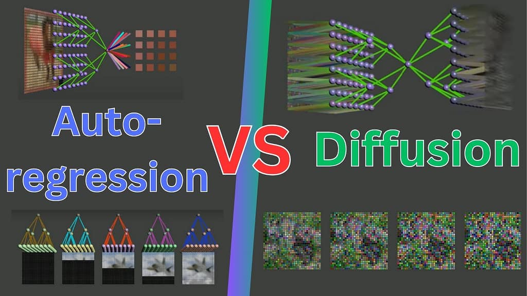
• Auto-regressive Models (Pixel-by-Pixel Generation):
  • To overcome the blurring problem, auto-regressive models approach image generation incrementally. Instead of generating an entire image at once, they predict one pixel at a time.
  • When predicting only one pixel, the average of possible values for that single pixel is still meaningful (e.g., the average of a bunch of colors is just another color, without blurring).
  • This process involves training separate neural networks for each pixel, or more practically, a single neural network that can predict a pixel’s value given a partially completed image and an indication of which pixel to generate.
  • The model learns to use previously generated pixels to inform its prediction for the next pixel, ensuring consistency.
  • Introducing Diversity: To make each generated image unique and creative, random sampling is incorporated. Instead of always selecting the label with the largest probability, the model randomly samples a value from the probability distribution of possible pixel values at each step. This randomness at each step influences subsequent predictions, leading to different outcomes each time.
  • Training Data: Auto-regressors are trained by taking original images and progressively removing pixels, then teaching the neural net to predict the missing pixels. The labels for training are the pixel colors from the original image itself, meaning no human labeling is required.
  • Limitations: While effective, auto-regressors are slow for images because they require evaluating a neural network once for every pixel (or element). Attempting to predict too many pixels at once reintroduces the blurring problem, as the model cannot ensure consistency between simultaneously predicted values. This problem is mitigated if the pixels being predicted are statistically independent, which is not the case for contiguous groups of pixels in natural images.
• Denoising Diffusion Models (Noise-based Generation):
  • Diffusion models improve upon auto-regression by changing the “removal process”. Instead of completely removing pixels, they add a small amount of random noise to the entire image. This is considered the most “spread-out” way of removing information, as it affects every pixel.
  • The neural network is then trained to undo this noising process, effectively “denoising” the image. While the model could predict the slightly less noisy image from the previous step, it’s often more effective to train it to predict the original, completely clean image or the noise that was added to the image.
  • By spreading out the information removal across the entire image through noise, the predicted values become as independent of each other as possible, which allows for fewer neural net evaluations and much faster generation of high-quality images compared to auto-regressors.
• Conditional Generation (e.g., Text-to-Image):
  • To generate images based on a text description (or other conditions like sketches), the neural network is simply given the text (or other conditioning input) as an additional input at each step of the generation process.
  • These models are trained on datasets containing pairs of images and their corresponding text descriptions, often scraped from the internet.
  • A technique called classifier-free guidance can further enhance the model’s adherence to the text prompt. During generation, the model is run twice: once with the text prompt and once without. The prediction without the prompt is then subtracted from the prediction with the prompt, helping to isolate and emphasize details derived from the prompt.

In essence, neural networks adapt curve fitting for image generation by breaking down the complex task into manageable prediction sub-problems (like predicting one pixel or denoising a noisy image) and then reassembling these predictions, often with the addition of randomness to introduce diversity and creativity.

Random sampling plays a crucial role in aiding creativity in neural networks for image generation by introducing diversity and uniqueness into the generated outputs.

Here’s how it works:

• The Problem Without Randomness: When a neural network, especially an auto-regressor, is trained to predict pixel values one at a time, if it simply outputs the label (e.g., pixel color) with the largest probability at each step, it will generate the exact same image every single time. The source notes that this is “not very creative”.
• Introducing Diversity through Probability Distributions: All predictors, including the neural networks used in image generation, actually output a probability distribution over possible labels for a given input.
• The Role of Random Sampling: Instead of always selecting the label that has the highest probability (which would lead to deterministic and identical outputs), random sampling involves randomly drawing a value from this probability distribution at each step of the generation process.
• Generating Unique Outcomes: Because a different value is sampled at each step, this randomness influences the subsequent predictions, leading to a “completely different image each time” the model is run. This mechanism transforms the model into an “interesting image generator”.

In essence, while the neural network still performs curve fitting to learn the underlying patterns and plausible pixel values, random sampling injects a non-deterministic element that allows for a multitude of valid interpretations and compositions, thus enabling the generation of novel and diverse images, rather than mere reproductions or averages.

Classifier-free guidance is a technique designed to make conditional diffusion models work better. It aims to enhance the model’s adherence to a given prompt, such as text.

Here’s how it works:

• Training Phase: During training, the model is sometimes given text prompts as an additional input, and sometimes it is not. This allows the same model to learn how to make predictions both with and without the conditioning prompt.
• Generation Phase: At each step of the denoising process (when the model is generating an image), the model is run twice:
  • Once with the prompt (e.g., the text description).
  • Once without the prompt.
• Guidance Calculation: The prediction made without the prompt is then subtracted from the prediction made with the prompt.
• Result: This subtraction process effectively removes details that would have been generated without the prompt, leaving only details that are directly derived from the prompt. This leads to generations that more closely follow the provided prompt.

Auto-regression is a method for image generation that adapts curve fitting by breaking down the complex task of generating an entire image into a series of simpler prediction steps, primarily focusing on one pixel at a time.

Here’s a breakdown of how auto-regression generates images:

• Addressing the “Blurry Mess” Problem:
  • If a neural network were trained to generate an entire image from a simple input (like a black image) all at once, it would produce a blurry mess. This is because if there are multiple plausible “labels” (i.e., different possible correct images) for the same input, the predictor learns to output the average of those labels. While averaging works for traditional classification tasks (e.g., 0.5 cat and 0.5 dog can still be a useful label), averaging a bunch of images or pixel values simultaneously does not result in a meaningful image; it just becomes blurry.
  • To overcome this, auto-regressors tackle the problem by predicting one pixel at a time. When predicting only a single pixel, the average of possible values for that pixel is still meaningful (e.g., the average of a bunch of colors is just another color), thereby avoiding the blurring effect.
• The Generation Process:
  • The core idea is to create a “removal process” that progressively removes pixels from an image, and then train neural networks to undo this process by generating and adding pixels back one at a time.
  • Initially, this was conceptualized as training a separate neural net for each missing pixel. For example, a model could be trained to predict the value of a single missing pixel, such as the bottom-right pixel of an image.
  • In practice, instead of using a different neural network for each step, a single neural network is used to perform all the generation steps. This model learns to predict the next pixel, given a partially completed image and potentially an indication of which pixel it’s supposed to generate.
  • The generation process begins with a completely black image, and the neural network progressively fills in one pixel at a time until a full image is formed.
• Introducing Creativity and Diversity:
  • If the model simply predicted the pixel value with the highest probability at each step, it would generate the exact same image every time, which is “not very creative”.
  • To introduce diversity, auto-regressors leverage the fact that all predictors output a probability distribution over possible labels. Instead of always selecting the label with the largest probability, the model randomly samples a value from this probability distribution at each step.
  • This random sampling ensures that each time the model is run, it samples different values, which in turn changes the predictions for subsequent steps, leading to a “completely different image each time”. This mechanism transforms it into an “interesting image generator”.
• Training Data:
  • The neural networks are trained on images where pixels are progressively removed, and the “labels” for the training are the pixel colors from the original image itself. This means that no human labeling is required, and models can be trained by simply scraping unlabelled images from the internet.
• Limitations for Image Generation:
  • Slowness: While auto-regressors can generate very realistic images, they are too slow for image generation. To generate an image, the neural network needs to be evaluated once for every element (pixel). Since large images can have tens of millions of pixels, this process takes an extremely long time.
  • Batch Prediction Issues: Attempting to speed up the process by generating multiple pixels (e.g., a 4×4 patch) at once can improve speed, but there’s a limit. If too many pixels are generated simultaneously, the model can’t ensure consistency between the simultaneously predicted values, leading back to the blurry mess problem where it averages many plausible ways to fill in a patch. This problem is particularly acute when predicting contiguous chunks of pixels, as nearby pixels in natural images are strongly related.
  • Due to these speed and quality trade-offs when trying to predict multiple pixels, auto-regressors are no longer commonly used to generate images.

Prediction tasks are a fundamental concept in neural networks, where a model is trained to predict a specific output or “label” given a particular input.

Here’s a breakdown of what prediction tasks entail:

• Training with Examples: In a prediction task, a neural network is provided with a training dataset composed of numerous examples, each containing an input and its corresponding correct label.
• Learning to Predict: The goal of the neural network is to learn the relationship between these inputs and their labels so that it can accurately predict the label for a new input it has not encountered before.
• Underlying Mechanism: Curve Fitting: Under the hood, the way prediction tasks are solved is by converting the training dataset into a set of points in a space. The neural network then fits a curve through these points. This is why prediction tasks are also known as curve-fitting tasks.
• Example: An example of a prediction task is training a neural network on images that are labeled with the type of object appearing in each image. Once trained, this neural network would be able to predict which object a human would identify in a new, unseen image.
• Distinction from “Generation” (Initially): While prediction is very useful, it’s initially seen as distinct from “generation” because it’s simply fitting a curve to existing points and not producing genuinely new content. However, as discussed, generative AI models like image generators are, in fact, just predictors that have been cleverly adapted for creative tasks.

Auto-regressors take too long to generate images primarily because of their sequential, one-element-at-a-time prediction process.

Here’s a breakdown of why this leads to slowness:

• Pixel-by-Pixel Generation: To generate an image, an auto-regressor needs to evaluate a neural network once for every element (pixel) in the image. This is a crucial distinction from traditional approaches that might try to generate an entire image at once and result in a “blurry mess” due to averaging multiple plausible outcomes. By predicting one pixel at a time, the model avoids this blurring effect, as the average of pixel colors is still a meaningful color.
• Millions of Evaluations for Large Images: While this sequential approach works for generating a few thousand words of text, large images can contain tens of millions of pixels. This means an auto-regressor would need to perform millions of neural network evaluations to complete a single image.
• Limitations of Batch Prediction:
  • To speed things up, one might try to generate multiple pixels, such as a 4×4 patch (16 pixels), at once. This could theoretically make generation 16 times faster.
  • However, there’s a limit to how many pixels can be generated simultaneously without degrading image quality. If too many pixels are predicted at once, the model encounters the original problem of averaging many plausible ways to fill in a patch, leading to a “blurry mess”.
  • The core issue is that when predicting a bunch of pixels simultaneously, the model cannot ensure consistency between the generated values. In contrast, when predicting one pixel at a time, the model can adjust its current prediction to be consistent with the previously generated pixels.
  • This problem is particularly pronounced because nearby pixels in natural images are strongly related. Knowing the value of one pixel often provides a good idea of what nearby pixels will be. Therefore, removing pixels in contiguous chunks (as one might do when trying to predict patches) is the least efficient way, as it forces the model to decide on strongly related values all at once, leading to a quality trade-off for speed.

Due to these speed and quality trade-offs when trying to generate multiple pixels simultaneously, auto-regressors are no longer commonly used to generate images, despite their ability to produce very realistic outputs. In contrast, diffusion models can achieve high-quality, photo-realistic images in about a hundred steps, significantly outperforming auto-regressors which would require millions of steps.

Classifier-free guidance is a technique designed to make conditional diffusion models work better. Its primary goal is to enhance the model’s adherence to a given prompt, such as a text description.

Here’s how it operates:

• Training Phase: During the training of the model, it is sometimes provided with text prompts as an additional input, and sometimes it is not. This method allows the same underlying model to learn how to make predictions both with and without the conditioning prompt.
• Generation Phase: When the model is actively generating an image (during each step of the denoising process), the model is executed twice:
  • Once with the prompt (e.g., the text description).
  • Once without the prompt.
• Guidance Calculation: The prediction that was made without the prompt is then subtracted from the prediction made with the prompt.
• Result: This subtraction effectively removes details that would have been generated even without the prompt, leaving only the details that are directly derived from and influenced by the prompt. This process leads to generated images that more closely follow the provided prompt.