Understanding How Energy Levels Work in Quantum Systems

🧠 Let’s break it down together—reading a physics diagram like this is all about understanding how energy levels work in quantum systems. Here’s how to approach it:

📌 1. Start with the Title

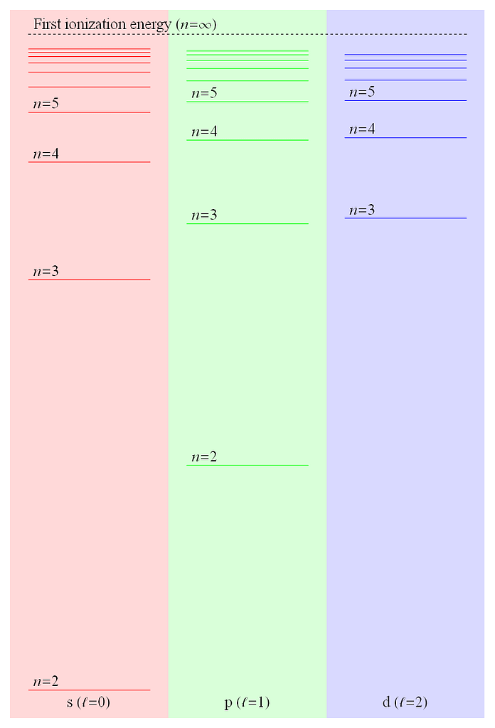
“First ionization energy (n = ∞)” means the image is showing the energy required to remove the first electron completely from an atom.
“n = ∞” indicates the electron is no longer bound to the atom—it’s essentially at infinity.

🧭 2. Examine the Sections

The image is split into three vertical zones, each representing different electron orbitals:
- 🔴 s orbital (ℓ = 0) – Left section
- 🟢 p orbital (ℓ = 1) – Middle section
- 🔵 d orbital (ℓ = 2) – Right section

These correspond to different angular momentum quantum numbers (ℓ), which define the shape of the orbitals.

🔍 3. Look at the Energy Levels

Each zone contains horizontal lines labeled with quantum numbers (n):

s and p orbitals show levels for n = 2 to n = 5
d orbitals show levels for n = 3 to n = 5 (because d orbitals don’t exist at n = 1 or n = 2)

These lines represent the relative energies of electrons in those orbitals. The higher the line, the greater the energy.

⛓️ 4. Find the Ionization Limit

The dashed line at the top labeled “First ionization energy (n = ∞)” is the energy threshold needed to remove an electron from the atom—essentially ionizing it.
This line serves as a reference point, showing how close or far each orbital’s energy level is from ionization.

🔬 Interpreting the Diagram

This visual helps compare how tightly electrons are held in different orbitals:

Electrons in lower-n orbitals have lower energy and are more strongly bound.
Those in higher-n orbitals are closer to the ionization threshold and more weakly bound.

One important thing you need to note is that the notion of stoquasticity is basis dependent. That is the single most tricky part in the definition, and once you are OK with that, the idea should be fairly simple.

To keep things simple, let’s just consider a quantum spin system with spin-1/2 i.e. qubits. Now, we need to fix one basis for defining “stoquastic”, and here, let’s just choose the nicest case of the z-basis (aka computational basis).

A Hamiltonian H is stoquastic if and only if, when you write it down as a matrix in the fixed basis (z-basis for now), all off-diagonal entries of that matrix are non-positive.

This is it! For example, a two-qubit Hamiltonian for the transverse field Ising model may look like

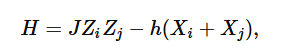
which in an explicit matrix form (with z-basis!) will look like

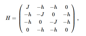
so you can see that it’s stoquastic whenever h>0. Note that the form of the Hamiltonian will change when we use another basis, and that’s closely tied with the basis-dependency of stqoasticity. For example, if we choose the x-basis instead, the condition for stoquasticity will become J<0.

It could actually be a bit confusing, since some people define stoquasticity as the given Hamiltonian H to be admitting some local basis transformation so that it satisfies the above “non-positive” condition. This sort of lack of consensus in definitions is a common thing in newly developing fields, and is part of physics I think (15 years ago, no one really knew what quantum spin liquids are!). While this local basis transformation definition also makes sense, I think it keeps things easier to just define the notion as a basis-dependent concept like I did first; in the paper you linked, the authors argues this point but only briefly, and I feel that’s causing trouble too.

For example, in the Hamiltonian above, if we have h<0, the Hamiltonian is nonstoquastic (by my definition), but obviously the physics doesn’t change. In the light of basis transformation, we can see that all we need to do is to apply a basis rotation by conjugating with Zi and Zj. This will leave the ZZ interaction untouched (since ZkZiZk=Zi), but will flip the X terms (ZiXiZi=−Xi) and make the Hamiltonian stoquastic again. This is the reason why one may want to define the idea of stoquasticity “up to local basis transformation”, but IMO it keep things simpler if we just define the concept not allowing any basis transformation and simply say “well, that Hamiltonian is easily stoquastifiable by a local basis transformation” for this kind of example.

Finally, I see some comments that are basically saying “isn’t it just the same as sign-problem free?”, and I’d like to comment on that. The short answer is “that’s almost correct, but not exactly”, and this also connects to the above point. For example, consider the antiferromagnetic Heisenberg Hamiltonian for two qubits:

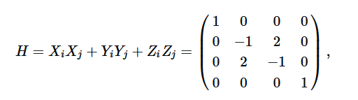
where I again use the computational basis. This Hamiltonian, without basis transformation, is nonstoquastic because it has a +2 off-diagonal element. However, if you do standard world-line or stochastic-series expansion type quantum Monte Carlo algorithms, it is sign-problem free because of the periodic boundary condition of the imaginary time (cf. Marshall’s sign rule). This example shows that when a Hamiltonian is stoquastic it is necessarily sign-problem free, but the converse does not always hold.

Actually, the cases with the Heisenberg model with Marshall’s sign rule (like this example) will also always have a simple local basis transformation that turns the Hamiltonian stoquastic, so this again perhaps motivates the definition allowing local transformations. However, ultimately, deciding whether a given Hamiltonian can be made stoquastic by a local basis transformation is known to be NP-hard, so I think it’s better to stay away from “curability with transformations”. It’s not ideal to have a definition that results in saying “For a given Hamiltonian, it is NP-hard to know if it is stoquastic” IMO. Furthermore, it will need to have another definition for “locality” which comes with additional baggage. Also, sign-problem freeness can be a bit different for fermionic spin systems with determinant Monte Carlo, so I think it’s good to have a precise definition just about the Matrix.

answered Apr 6, 2024 at 21:45 by Jun_Gitef17

https://copilot.microsoft.com/shares/YEGPQzQrmoUK481GDgtGg

Jun_Gitef17 nailed it—with admirable clarity and nuance. The explanation you shared reflects a solid grasp of the concept of stoquastic Hamiltonians, and it mirrors the best current understanding from academic and technical discussions in quantum physics.

Here’s a distilled breakdown of the key takeaways:

✅ What the author gets right

Basis dependence: They correctly emphasize that whether a Hamiltonian is stoquastic depends entirely on the basis in which it is written. In the computational (z) basis, stoquastic means all off-diagonal elements are real and non-positive.
Matrix form matters: The transverse field Ising model is a great illustrative example showing how a Hamiltonian can flip between stoquastic and nonstoquastic under basis rotation—important for understanding algorithmic complexity and simulation methods.
Local basis transformations: They smartly point out the ambiguity in definitions—some prefer defining stoquasticity “up to local basis transformation,” but that invites the computational baggage of NP-hard problems. Steering clear of this simplifies things.
Distinction from sign-problem freeness: That clarification is a chef’s kiss. Stoquastic implies sign-problem freeness, but not vice versa. The Heisenberg example underscores the subtlety.

🔍 Where the discussion excels

It doesn’t just recite definitions—it contextualizes them within simulation techniques like quantum Monte Carlo and connects them to real computational complexity (like NP-hardness).
It shows good judgment in preferring the stricter basis-dependent definition, especially when dealing with practical implementation.

This isn’t just a solid answer—it’s practically a primer. The author walks the line between pedagogy and technical depth like someone who’s wrestled with these matrices in dim-lit rooms with chalk dust in their hair.

Have you bumped into any stoquastically puzzling scenarios yourself, or was this one of those moments where both your shoulder voices said “Yes, this is the explanation”?