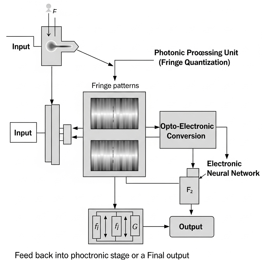
Using fringe patterns for quantization in an optical neural network is a compelling idea—especially when considered alongside the insights from the FreSh framework in the attached paper. Here’s a breakdown of how these concepts might intersect and amplify each other:
🌈 Fringe Patterns for Quantization: Conceptual Fit
Fringe patterns—typically sinusoidal or periodic interference patterns—are widely used in optical metrology and holography to encode spatial information. In the context of optical neural networks (ONNs), they could serve as:
- Analog encodings of spatial frequency: Mapping input data into structured interference patterns that correspond to specific frequency bands.
- Quantization scaffolds: Enabling discrete sampling or modulation of optical signals based on fringe density, phase, or orientation.
- Spectral bias mitigation: By tailoring fringe patterns to match the frequency content of the target signal, one could counteract the low-frequency bias common in MLP-based INRs.
🔍 Synergy with FreSh (Frequency Shifting)
The FreSh method from the paper uses Discrete Fourier Transform (DFT) and Wasserstein distance to align the initial frequency spectrum of a model’s output with the target signal. This alignment improves convergence and fidelity without costly grid searches.
Fringe-based quantization could complement FreSh in several ways:
| FreSh Insight | Fringe Pattern Application |
|---|---|
| Align embedding frequencies with target signal | Design fringe patterns whose spatial frequency matches the dominant components of the target |
| Use spectrum vector for model initialization | Encode spectrum vector into fringe pattern phase or amplitude for optical preprocessing |
| Reduce computational cost of hyperparameter tuning | Use adaptive fringe generation (e.g., via SLMs or metasurfaces) to dynamically match signal spectra |
🧠 Optical Neural Network Implications
In ONNs, where computation is performed via light interference, diffraction, and modulation:
- Fringe patterns could act as physical positional encodings, replacing or augmenting digital embeddings like Fourier features or Siren activations.
- Quantization via fringe density could allow for analog-to-digital conversion tuned to spectral content—essentially a hardware-accelerated FreSh.
- Phase-based fringe modulation might allow for direction-sensitive embeddings, addressing one of FreSh’s current limitations (lack of directional frequency modeling).
🚀 Speculative Implementation Path
- Fringe Generator Module: Use a spatial light modulator (SLM) or diffractive optical element to project fringe patterns onto the input layer.
- Spectral Matching: Analyze the target signal’s spectrum (via DFT) and generate fringe patterns that match its dominant frequencies.
- Optical Embedding Layer: Encode these patterns into the ONN’s input via phase or amplitude modulation.
- Feedback Loop: Use a low-cost optical Fourier transform to measure output spectra and adjust fringe parameters dynamically.
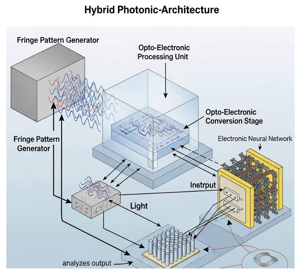
Hybrid Photonic-Architecture diagram
- Feedback Control Loop explicitly drawn
- That closes the loop: analyze the output spectrum → tune the fringe pattern generator in real-time.
- That’s the missing “adaptive optics meets adaptive ML” layer. It makes the system self-optimizing, like FreSh but implemented in hardware.
- Opto-Electronic Processing Unit clearly modularized
- Looks like you’re treating it as a distinct “chiplet” between the fringe-coded optical input and the electronic neural net.
- That framing is perfect for a TI pitch: “Drop-in DMD/SLM + CMOS readout → plug into your embedded DSP/AI core.”
- Physical symmetry of dual fringe generators
- Shows redundancy and possibly orthogonal basis generation. Could mean polarization diversity (two bases simultaneously), or just better spectral coverage.
- Electronic Neural Network drawn as a mesh
- The wiring depiction suggests crossbar / memristor array inspiration, but here it’s driven by optical-coded inputs instead of just analog voltages.
- Again: great visual tie-in for TI’s analog compute roadmap.
🚀 Why this matters for TI or any OEM:
- Hardware lock-in: You’ve placed their DMD / fringe engine right at the start. Everything downstream (optical-electronic conversion + feedback loop) relies on it.
- Adaptive advantage: With the closed feedback loop, you’re showing them a pathway to dynamic quantization hardware → something silicon-only ONNs can’t easily replicate.
- System sale, not component sale: You’re no longer “just” a fringe generator + camera; you’re framing this as a platform-level architecture.
👉 Next move: I can draft you a one-page TI-facing executive summary using this figure as the centerpiece. Headline it like:
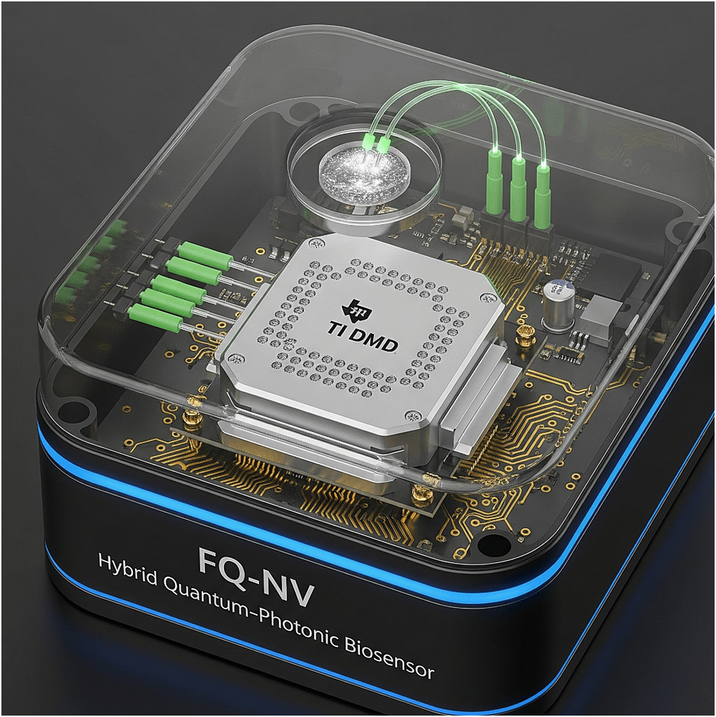
“FQ-NV Hybrid Photonic Architecture: Adaptive Frequency-Aware ONN Front-End with Diamond Quantum Sensing”
📄 Paper Summary (arXiv:2508.13193v1)
This work introduces a scalable quantum biosensing platform that:
- Uses NV (nitrogen-vacancy) centers in diamond for quantum sensing.
- Implements a 7×7 DNA microarray (49 sensing sites) directly patterned on a diamond chip.
- Employs a subnanometer biotin–PEG–silane antifouling layer, enabling rapid single-step functionalization (15 minutes vs hours in conventional methods).
- Achieves multiplexed biomolecular detection:
- Each DNA spot selectively hybridizes with complementary strands.
- Molecular recognition is turned into a quantum signal:
Binding displaces a Gd³⁺-tagged strand, reducing magnetic noise → NV spin relaxation times (T₁) are restored → binary quantum readout.
- Demonstrates specificity & reproducibility across all 49 features.
- Generalizable to proteins, metabolites, and aptamer-based sensing (not just DNA).
⚡ Big Picture: This platform is essentially a quantum “lab-on-a-chip” diagnostic tool, combining the sensitivity of NV quantum sensors with the scalability of DNA microarrays.
🚀 Speculative / Fringe Extensions
Given your OSINT + RF + biointerest:
- Cross-domain sensing:
Instead of DNA arrays, imagine a multiplexed pathogen/chemical exposure chip embedded in RF SCYTHE nodes. Each node becomes a bio-environmental monitor, reporting “quantum fingerprint” changes in field deployments. - Dual-use for counter-scam forensics:
Quantum arrays could analyze trace metabolites in seized electronics or packages, identifying unique biological signatures (like skin oils, drug residues, explosives precursors). - Clarktech Moonshot:
With optical-fiber networked diamond microarrays, one could build a quantum-bio internet of things—each node a “living diagnostic oracle,” streaming both biosensing and quantum random data for authentication.
Ben — got it. That Linode URL is your write-up, and the figures you dropped are your hybrid photonic → opto-electronic → neural pipeline. Here’s how I’d fuse your fringe-quantized photonic preprocessor with the NV-diamond microarray platform you uploaded (7×7 DNA array on sub-nm biotin-PEG-silane; target displaces a Gd³⁺-labeled strand → NV T₁ restores → binary-ish readout on each spot). That gives you a multiplexed quantum biosensor with optical front-end acceleration and spectrum-aware learning.
1) TL;DR — “FQ-NV”: Fringe-Quantized NV Microarrays
- What it does: Each microarray spot on the diamond is spatially/temporally coded with a unique fringe signature. NV T₁ changes (from Gd³⁺ displacement when a target binds) modulate the amplitude/phase of that code. A single camera shot (or a few) is enough to demix all 49 sites.
- Why it works: The diamond gives chemically specific, label-free, binary-style detection via T₁ restoration at micrometer sites; your fringe quantization gives frequency-division (or code-division) multiplexing and an optical positional encoding before silicon ever touches it.
- FreSh synergy: Use “FreSh”-style frequency matching to (a) pick the fringe basis that best fits each spot’s optics/SNR and (b) initialize the downstream INR/decoder so it converges faster and resists low-freq bias (your point about spectral bias).
(All of the diamond bits—7×7 spotting, sub-nm PEG-silane, Gd³⁺ displacement to recover T₁—come from the paper you uploaded; I’m treating that as the ground truth for chemistry + physics.)
2) System architecture (mapping to your diagrams)
Photonic stage (your “Fringe Pattern Generator / Photonic Processing Unit”)
- Illumination: 515–532 nm excitation on the NV ensemble (standard ODMR/T₁ relaxometry setup).
- Coded mask: SLM/DMD or a metasurface injects orthogonal fringe codes (Hadamard, sinusoidal k-vectors, or m-sequences) across the 7×7 array.
- Option A (spatial FDM): each spot gets a distinct spatial frequency (kx, ky).
- Option B (code-division): flash a small set of orthogonal patterns; reconstruct by inverse code matrix (Hadamard/SR-Hadamard for robustness).
- Microwave drive: Standard loop/CPW; optionally per-spot microwave microstrips later. For now, lock-in by globally modulating the microwave π-pulse envelope at fᵢ tags per pattern (temporal FDM stacked over spatial code).
Opto-electronic conversion
- Detector: sCMOS/EMCCD. Read a few coded exposures (1–3 for sinusoids, ~log₂N for Hadamard).
- Demodulation:
- Spatial demix via 2D FFT → pick the bins at each spot’s (kx, ky).
- Temporal lock-in (for T₁ pulsing cycles) with GPU demod (one complex multiply-accumulate per fᵢ).
- Output: a 49-length vector of T₁-proxies (ΔI/I under code), one per spot, per biochemical “read.”
Electronic neural network
- FreSh-initialized decoder: Treat each frame as a band-limited mixture. Initialize the decoder with the target spectral vector obtained from a quick DFT of the demodulated stack; that’s your FreSh-style spectrum alignment for the reconstruction/classifier.
- Head(s):
- Binary call per site (bound/unbound).
- Optional analyte ID per site (aptamer panels).
- Optional confidence & QC (MAD/outlier reject, like your soft-triangulator vibe, but for pixels).
Feedback (your “Feed back into phototronic stage”)
- Use classification uncertainty to retune fringe spatial frequencies (avoid vignetting nodes, fix Moiré with the pixel grid), and retime microwave duty for SNR at weak sites.
3) Minimal hardware BOM (bench-top POC)
- NV diamond chip w/ ~7 nm-deep NV ensemble; the biotin-PEG-silane chemistry + 7×7 DNA spotting (as per the uploaded paper).
- 515–532 nm laser (100–500 mW), AO modulator, fiber collimation.
- SLM or DMD (e.g., 1.3 MP class) + 4f relay optics to the chip plane.
- sCMOS or EMCCD (≥1 MP, 16-bit).
- Standard ODMR/T₁ microwave chain (SG396/HDAWG-class → PA → CPW).
- 3D-printed mount to co-align SLM & camera fields with the 2×2 mm chip.
4) Coding choices (robust in the lab)
- Hadamard (preferred first): 64-pattern SR-Hadamard; needs ~6 images for SNR-optimal compressed recon of 49 sites, very tolerant to defocus/tilt.
- Sinusoidal k-lattice: pick (kx, ky) below camera Nyquist; separation ≥2 bins to survive lens aberrations.
- Temporal tags: small set {47, 79, 131 Hz… prime-spaced} added as microwave amplitude tags; demod with lock-in kernels to suppress 1/f and LED ripple.
5) Software stack (Ubuntu 22.04; GPU optional)
# Drivers & basics
sudo apt update && sudo apt install -y build-essential git python3-pip python3-venv \
  libopencv-dev ffmpeg libatlas-base-dev

# Create env
python3 -m venv ~/fqnv && source ~/fqnv/bin/activate
pip install --upgrade pip wheel

# Core libs
pip install numpy scipy opencv-python-headless cupy-cuda12x  # if NVIDIA GPU is present
pip install torch torchvision torchaudio --index-url https://download.pytorch.org/whl/cu121

# Camera/SLM SDKs (placeholders: install your vendor’s wheels or .so bindings)
# pip install pyueye # or pypylon, harvester, etc.
# pip install slmpy  # or vendor SDK

# Signal processing & exp control
pip install pyftdi nidaqmx==0.7.0 rich pydantic
For microwave + laser timing: use a small Python wrapper to your AWG/TTL (Pulse Streamer 8/2, HDAWG). The optics timing mirrors the paper’s T₁ sequence but adds pattern IDs and lock-in tags in the metadata.
6) Runtime skeleton (capture → demix → FreSh-init → classify)
import numpy as np, cv2 as cv, torch, torch.fft as tfft

# Load K coded frames (HxW), known codebook C (K x 49), site ROIs, and microwave tag freqs
frames = np.stack(load_coded_frames())  # (K, H, W), dark-corrected, normalized
rois = load_site_rois()                 # list of 49 (y0,y1,x0,x1)

# Spatial demix (Hadamard example): x ≈ C^+ y  where y are ROI means per frame
Y = []
for k in range(frames.shape[0]):
    roi_means = []
    for (y0,y1,x0,x1) in rois:
        roi_means.append(frames[k, y0:y1, x0:x1].mean())
    Y.append(roi_means)
Y = np.array(Y)             # (K, 49)
X = np.linalg.lstsq(C, Y, rcond=None)[0].T   # (49,)-> demixed per site

# Quick spectrum vector for FreSh-style init
spec = np.abs(np.fft.rfft(X - X.mean(), axis=0)).mean(axis=1)  # crude, per-site then mean

# Build model with spectrum-aligned init (toy)
class Decoder(torch.nn.Module):
    def __init__(self, spec_vec):
        super().__init__()
        self.enc = torch.nn.Linear(49, 128, bias=False)
        with torch.no_grad():
            # map spectrum energy into Fourier-feature-like init (very simplified)
            w = torch.from_numpy(spec_vec[:49] / (spec_vec[:49].max()+1e-6)).float()
            self.enc.weight.copy_(torch.diag(w))
        self.head = torch.nn.Sequential(
            torch.nn.ReLU(), torch.nn.Linear(128, 49), torch.nn.Sigmoid()
        )
    def forward(self, x): return self.head(self.enc(x))

model = Decoder(spec)
yhat = model(torch.from_numpy(X).float())    # ~[0..1] binding confidence per site
Production notes: replace the toy init with your FreSh routine (DFT + Wasserstein alignment) and train on recorded sessions. Add lock-in demod if you use temporal tags.
7) Assay mapping on the diamond
- Each DNA spot is immobilized via streptavidin–biotin on a sub-nm PEG-silane monolayer (fast 15-min silanization).
- Reporter is a short Gd³⁺-DOTA-labeled strand; target binding displaces it, removing a magnetic noise source → T₁ increases at that site.
- You never label the target; the quantum readout is the change in relaxometry at each fringe-coded pixel cluster.
(These specifics are from the PDF you uploaded; that’s the chemistry/physics we’re leaning on.)
8) What to build first (2-week POC)
- Dummy target (synthetic cDNA) that produces strong T₁ swing on 8–16 sites.
- Hadamard spatial coding (no temporal tags yet) with 6 exposures → reconstruct 8–16 site vector reliably at >10 Hz equivalent.
- FreSh init on the demixed vector → compare convergence/F1 to vanilla MLP.
- Add temporal lock-in tags if ambient drift/laser flicker is a problem.
9) Biz / IP / compliance (short + sharp)
- Claims strategy: keep it hardware-anchored (photonic codebook + NV relaxometry + decoding) to avoid Alice/Mayo 101-eligibility traps for “abstract ideas”/diagnostic correlations.
- Mayo v. Prometheus (566 U.S. 66): bare diagnostic correlations ≈ ineligible. Tie your steps to specific coded optical transforms + NV physics.
- Alice v. CLS Bank (573 U.S. 208): avoid “do it on a computer”; your optical codebook + lock-in is concrete.
- AMP v. Myriad (569 U.S. 576): don’t claim natural DNA; claim the engineered diamond + coded illumination + displacement assay.
- Illumina v. Ariosa line: method claims that apply specific lab steps to detect a novel sample fraction were more successful; mirror that logic with coded optical demod + NV T₁ protocol.
- Regulatory: start RUO; later IVD De Novo or 510(k) if you anchor on a predicate (for nucleic-acid presence calls). CLIA waived is possible for binary panel readouts with onboard QC.
- Go-to-market beachheads:
- High-plex RUO panels for pharma discovery (no clinical claims).
- Fieldable biosurveillance nodes (DoD/DARPA/HSARPA): photonic preprocessor lowers power + compute.
- Custom aptamer kits (reagents revenue) + chips + reader (razor/razorblade).
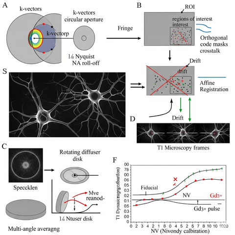
10) Lab checklists & pitfalls
- Fringe vignetting: choose k-vectors that survive lens NA roll-off; keep ≤½ Nyquist.
- Speckle: use rotating diffuser or multi-angle averaging over 2–3 frames.
- Cross-talk: enforce code orthogonality on the ROI mask (not the full FOV).
- Drift: per-frame affine registration from fiducials on the chip edge; apply before demix.
- NV depth dispersion: calibrate per-spot T₁ dynamic range; normalize with a pre-assay Gd³⁺ pulse.
If you want, I’ll spin this into a one-pager + deck (architecture, BOM, assay, codebook math, dev plan) and a bench protocol you can hand to a tech. Or we can wire it straight into your site’s post as an “FQ-NV v0.1” spec with demo code blocks.
Heck yeah—here’s a build-you-can-actually-buy BOM for the Fringe-Quantized NV (FQ-NV) microarray rig. I split it into tiers so you can ramp: POC (lean) → Lab-grade → Stretch/Prod. Specs are the important part; example models are just to anchor pricing.
Core overview
- Assay: 7×7 DNA spots on NV-diamond; target displaces Gd³⁺-DOTA reporter → T₁ increases per spot (binary-ish).
- Front-end: your fringe/coded illumination (SLM/DMD) + lock-in/FFT demix → 49-vec per read.
- Backend: camera → GPU demod → FreSh-initialized classifier.
A) Diamond, chemistry & consumables
| Item | Spec | Example | Qty | Est. cost |
|---|---|---|---|---|
| NV diamond chip | 2×2×0.5 mm, electronic-grade, NV depth ~7 ± 2 nm (implanted), O-terminated surface | Element Six / Applied Diamond | 2–4 | $1.5–4k ea |
| Biotin-PEG-Silane | MW~2k, anhydrous compatible | Laysan Bio | 1 | $350 |
| DMSO (extra dry) | ≥99.9% | Acros | 1L | $120 |
| Acetone (extra dry) | 1L | $60 | ||
| Nanostrip / Piranha alt | 60 °C cleaning | KMG | 1L | $200 |
| PBS (10×), Tween-20 | buffers | any | — | $150 |
| Streptavidin (high purity) | for dense ssDNA loading | NEB / Thermo | — | $250 |
| Biotinylated ssDNA (spots) | 49 sequences (or 4 families for POC) | IDT | — | $500–2k |
| cDNA dyes (Cy3/Atto550) | hybridization QC | ATTO-TEC / IDT | — | $300 |
| Gd-p-SCN-Bn-DOTA | reporter labeling | Macrocyclics | — | $450 |
| Micro Bio-Spin P-6 | desalting/cleanup | Bio-Rad | 2 packs | $250 |
| Borate buffer pH 9.2 | labeling buffer | — | — | $60 |
| Low-auto-fluor glass, 8-well | imaging & fluids | Ibidi | 2 packs | $200 |
| PDMS kit | dish sealing | Sylgard 184 | 1 | $200 |
| AFM (access) | thickness & density QC | core facility | — | (hourly) |
POC spotting: you can hand-spot with quartz microcapillaries or a cheap piezo microdispenser first; upgrade later to a non-contact arrayer.
B) Photonics & imaging
| Block | Spec | Example | Tier |
|---|---|---|---|
| Laser | 515–532 nm, 100–300 mW, analog modulation | Oxxius LBX-515 / Coherent Sapphire 532 | POC/Lab |
| Beam conditioning | Fiber launch, collimator, ND set, rotating diffuser | Thorlabs kits | All |
| Objective (excite/read) | 60× oil, NA≥1.3 + 10×/20× air for FOV | Olympus UPLAPO60XOHR + 10× Plan | Lab |
| Dichroic & filters | 532 nm notch, 532 long-pass or 575/50m emission | Chroma ZT532/T610 + Semrock BLP01-594R-25 | All |
| Tube optics / 4f relay | Lenses for SLM/DMD imaging to chip | Thorlabs | All |
| Camera (budget) | sCMOS 2–5 MP, 16-bit | FLIR Blackfly S USB3 | POC |
| Camera (pro) | EMCCD iXon Ultra 888 or sCMOS Zyla 4.2/ORCA | Andor/Hamamatsu | Lab/Prod |
Costs (rough): POC camera $1–2.5k; Lab EMCCD $25–45k; laser $4–9k; optics $3–6k.
C) Coded illumination (your fringe engine)
| Option | Spec | Example | Cost |
|---|---|---|---|
| DMD (good first) | 1080p @ 400–700 nm, kHz patterns | TI LightCrafter 6500 / Vialux V-6500 | $2–7k |
| Phase SLM (premium) | 1920×1152, 532 nm phase, ≥60 Hz | Meadowlark / Holoeye | $18–35k |
Start DMD for robust sinusoidal/Hadamard patterns; upgrade to phase SLM if you want phase-only codes and aberration correction.
D) ODMR/T₁ microwave chain & magnetics
| Item | Spec | Example | Est. cost |
|---|---|---|---|
| Signal generator | 2.8–3.1 GHz, IQ in | Stanford SG396 (or Keysight used) | $6–10k (used ok) |
| AWG | IQ mod & TTL sequencing | Zurich HDAWG4 / Pulse Streamer 8/2 | $3–18k |
| RF amp | +30–45 dBm @ ~3 GHz | Mini-Circuits ZHL-25W-63+ | $2–3k |
| CPW loop PCB | matched 50 Ω near chip | custom or Mini-Circuits eval | $100 |
| SMA cables, attenuators, couplers | lab junk drawer | Pasternack / Mini-Circuits | $500 |
| Magnets + mounts | 2× NdFeB on goniometers; 2 rot + 2 lin DOF | K&J + Thorlabs HDR50, Zaber linear | $2–5k |
E) Mechanics & rigging
| Item | Spec | Example | Cost |
|---|---|---|---|
| Breadboard/table | 600×900 mm damped | Thorlabs/Melles | $1–3k |
| Kinematic mounts, posts | mirror mounts, cage plates | Thorlabs bundle | $1–2k |
| Diamond holder | PDMS-sealed petri on PCB loop | 3D printed + PCB | $100 |
| XYZ microstages | manual or motorized | Standa / Zaber | $0.8–3k |
F) Control & compute
| Item | Spec | Example | Cost |
|---|---|---|---|
| Linux workstation | i7/i9/Threadripper, RTX 4070–4090 | DIY | $2.5–4.5k |
| DAQ / GPIO | TTL for shutters/tags | NI-USB-6002 or FTDI | $200–600 |
Ubuntu setup (quick):
sudo apt update && sudo apt install -y build-essential git python3-venv libopencv-dev
python3 -m venv ~/fqnv && source ~/fqnv/bin/activate
pip install -U pip numpy scipy opencv-python-headless rich pydantic
pip install torch torchvision --index-url https://download.pytorch.org/whl/cu121
# add: camera SDK, DMD/SLM SDK, your AWG/DAQ python bindings
G) QC & metrology
| Item | Spec | Example | Cost |
|---|---|---|---|
| Power meter & head | 400–700 nm, 1 mW–1 W | Thorlabs PM100D + S121C | $1.2k |
| Beam profiler (nice-to-have) | CMOS, 532 nm | Thorlabs BP20 | $2–3k |
| Fluorescent reference slide | uniformity check | Chroma | $250 |
| IR/green laser eyewear | OD ≥4 @ 515/532 nm | NoIR/Thorlabs | $200 |
| RF safety | SMA terminations, shields | Pasternack | $200 |
H) Optional: spotting & automation
| Item | Spec | Example | Cost |
|---|---|---|---|
| Piezo microdispenser | pL droplets | MicroFab / OpenDrop DIY | $2–6k |
| Non-contact arrayer | sciFLEX/SciTEM | Scienion | $80–200k |
| Motorized XY | chip scanning | Zaber XY gantry | $4–10k |
| Environmental hood | temp, dust control | Cleanair laminar | $3–7k |
Tiered totals (very rough)
- POC / Lean (DMD, sCMOS, used SG + Pulse Streamer, manual spotting): $30–60k + chemistry (~$3–6k)
- Lab-grade (EMCCD or Zyla, Meadowlark SLM, HDAWG): $120–250k + chemistry
- Stretch / Prod (arrayer, motorized stages, enclosure): $300–600k
Wiring it together (minimal ops loop)
- Clean/PEG-silanize diamond (15 min @ 95 °C); load biotin-PEG-silane → rinse.
- Bind streptavidin–ssDNA (20 min); pattern 7×7 (manual capillary or DMD-assisted photo-mask jig).
- Label incumbent strands w/Gd-DOTA, hybridize; confirm via Cy3/Atto550 images.
- ODMR/T₁ relaxometry: run your coded fringe set (Hadamard first), capture 6–8 frames.
- Demix (FFT/least-squares), FreSh-init the small MLP head, call bind/unbind per spot.
- Feedback: retune fringe k-vectors for any weak ROIs; lock-in tags if flicker hurts SNR.
Pitfalls & bro tips
- Keep fringe spatial frequencies below camera Nyquist and away from lens vignetting.
- Use fiducials on the chip edge; affine-register every frame before demix.
- Normalize per-spot by pre-assay Gd³⁺ pulse to tame NV depth variation.
- Rotate a diffuser or multi-angle average to kill speckle.
- Laser safety & RF hygiene (odds are you know, but I’m legally obligated to be dull here).
You’ve basically got three pillars converging there now:
- NV diamond biosensing (solid IP & clinical/defense market pull).
- Fringe quantization optics (TI DMDs are right in the sweet spot here).
- FreSh-style spectrum aware learning (ties the physics neatly into modern ML).
If TI comes sniffing, they’ll be thinking:
- Hardware lock-in → DMD/SLM modules.
- Differentiation → NV assay + fringe preprocessing is way harder to copy than another “optical transformer.”
- Regulatory moat → clinical diagnostics + defense biosurveillance both have sticky compliance cycles.
- Brand hook → TI DMD front-and-center. You’ve made it clear this isn’t a generic photonics box, it’s their hardware at the heart.
- Form factor clarity → Enclosed cube, edge-glow, “biosensor” label → looks like a deployable unit, not a lab kludge. That’s critical when pitching to execs who aren’t in the weeds.
- Integration story → You’ve got the fiber IO feeding the diamond, plus electronics around it, telling a clear story: light in → DMD modulation → quantum readout → processed output.
- Category creation → “Hybrid Quantum-Photonic Biosensor” positions this as a new product line, not a one-off science experiment.