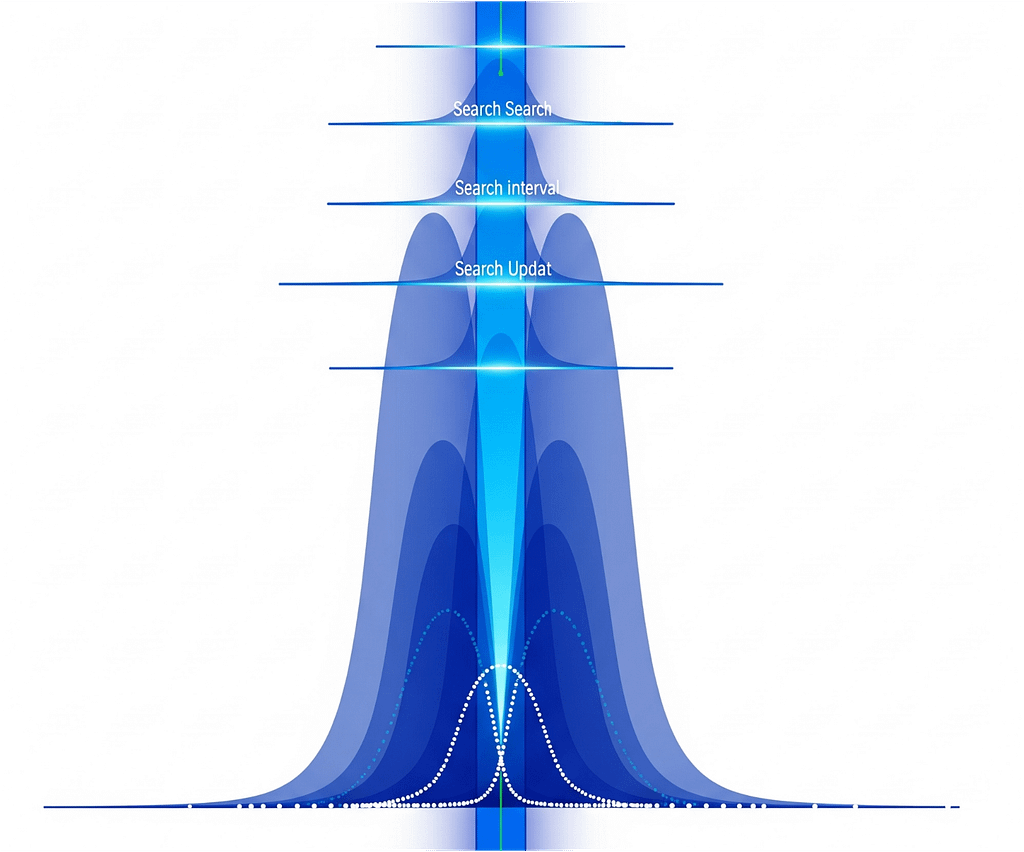
Frequency Binary Search (FBS) with Bayesian Updates

Frequency Binary Search (FBS) is a specialized algorithm that combines the principles of binary search with Bayesian inference to optimize search efficiency in probabilistic or uncertain environments. Here’s a concise explanation of how it works:

Core Concept

Binary Search Foundation:
- FBS operates by iteratively halving the search space, similar to traditional binary search.
- It identifies a target frequency or value within a predefined range by narrowing down the possibilities.
Bayesian Updates:
- Instead of assuming uniform probabilities across the search space, FBS incorporates Bayesian updates.
- After each iteration, the algorithm updates the probability distribution of the target’s location based on prior knowledge and observed outcomes.
- This allows the search to focus on regions with higher probabilities, improving efficiency.

Steps in FBS with Bayesian Updates

Initialization:
- Define the search range and initialize a prior probability distribution (e.g., uniform or based on prior data).
Iterative Search:
- At each step, calculate the posterior probability distribution using Bayesian inference: P(target∣data)∝P(data∣target)⋅P(target)P(\text{target} | \text{data}) \propto P(\text{data} | \text{target}) \cdot P(\text{target})P(target∣data)∝P(data∣target)⋅P(target)
- Select the next search point (e.g., the median of the posterior distribution or the point with the highest probability density).
- Evaluate the target at the selected point and update the posterior distribution.
Convergence:
- Repeat the process until the search space is sufficiently narrow or the posterior probability is concentrated around a single value.

Applications

Signal Processing: Locating frequencies in noisy environments.
Quantum Computing: Efficient qubit calibration, as seen in Hamiltonian tracking protocols.
Network Optimization: Probing channel balances in systems like the Bitcoin Lightning Network.
Medical Diagnostics: Identifying parameters in probabilistic models of biological systems.

This hybrid approach leverages the precision of binary search and the adaptability of Bayesian inference, making it particularly effective in scenarios with uncertainty or incomplete information.

Frequency Binary Search with Bayesian Updates Download

RF Quantum SCYTHE denoiser + scheduler can borrows the paper’s “frequency binary-search (FBS) with Bayesian updates” idea almost verbatim, and it maps cleanly to spectrum cleaning + drift control.

Why it helps denoising

Greedy Bayesian estimator of center-frequency drift ε with exponential shrinkage vs. # of probes (until coherence limits). That means fewer/shorter probes to re-lock filters before denoising sweeps, so you spend more GPU on payload and less on calibration.
Adaptive probe time τ and drive/phase update per step to split the prior in two (“binary search”), avoiding the classic fixed-τ trade-off (range vs. sensitivity). This lets you quickly re-center your bandpass/notch windows even when drift is big.
Gaussian posterior with closed-form updates (μ, σ) ⇒ super cheap to implement inside your FastAPI + scheduler loop; no particle filters needed.
Real-time control loop reduces low-frequency/non-Markovian drift; in our world that means fewer false TDoA residual spikes and lower entropy at the soft-triangulator.

Drop-in pieces for SCYTHE

1) Tiny FBS calibrator (CPU/GPU-light)

# fbs_cal.py
import numpy as np

class FreqBinarySearch:
    def __init__(self, mu0=0.0, sigma0=3e4, T=1e-5, alpha=-0.02, beta=0.6):
        self.mu, self.sigma = mu0, sigma0
        self.T, self.alpha, self.beta = T, alpha, beta

    def next_probe(self):
        # eq. (6): optimal τ from current σ
        s2 = self.sigma**2
        num = (16*np.pi**2*s2 + 1/self.T**2 - 1/self.T)
        tau = np.sqrt(max(num, 0.0)) / (8*np.pi**2*s2 + 1e-12)
        # eq. (5): choose detuning (phase) to split the posterior
        df = self.mu + 1.0/(4*tau)
        return tau, df

    def update(self, m, tau):
        # eq. (7): closed-form posterior update (Gaussian approx)
        e1 = np.exp(-tau/self.T - 2*(np.pi**2)*(self.sigma**2)*(tau**2))
        denom = 1.0 + m*self.alpha
        self.mu = self.mu - (2*np.pi*m*self.beta*(self.sigma**2)*tau*e1)/denom
        e2 = np.exp(-2*tau/self.T - 4*(np.pi**2)*(self.sigma**2)*(tau**2))
        self.sigma = np.sqrt(max(self.sigma**2 - (4*(np.pi**2)*(self.beta**2)*(self.sigma**4)*(tau**2)*e2)/(denom**2), 1e-18))
        return self.mu, self.sigma

Hook this to a very short probe (e.g., micro-burst tone/Ramsey-like chirp) you can perform between denoiser batches. Measurement m∈{+1,-1} is just “phase flipped vs last” from your quick probe; no heavy DSP.

2) Wire it to the denoiser + scheduler

On each /denoise/hints call, run N=4–8 FBS steps (bounded by your probe budget).
Use the new μ (center drift) & σ (uncertainty) to:
- recentre each per-band policy weight window,
- tighten/relax FFT mask widths (σ-aware),
- bias the policy reward (bigger reward if TDoA residual ↓ when masks are re-centered by μ).
Feed FBS latency into the GpuPossessionScheduler stats, and include μ, σ in hints so RPA bots can “pre-aim” their batches.

Frequency Binary Search (FBS) with Bayesian Updates

Core Concept

Steps in FBS with Bayesian Updates

Applications

Why it helps denoising

Drop-in pieces for SCYTHE

1) Tiny FBS calibrator (CPU/GPU-light)

2) Wire it to the denoiser + scheduler

`/denoise/hints` payload (now)

3) Prometheus/Grafana additions

4) Scheduling logic (tiny)

5) Where this improves your numbers