Recovering Dynamics from Energy Bands: A Sparse Regression Approach 🧠

Let’s unpack the function recover_ode for a technically curious audience, especially those working in signal processing, sparse modeling, or data-driven dynamical systems:

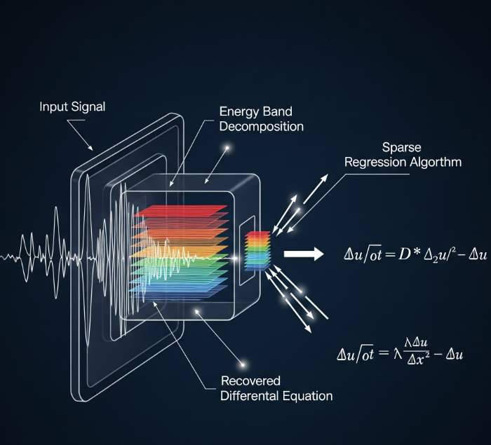
In many signal processing and physics-inspired machine learning tasks, we’re often handed a time-frequency representation—say, a matrix of energy across frequency bands over time—and asked to infer the underlying dynamics. What drives the changes? Can we recover a differential equation that governs the system’s evolution?

Enter recover_ode: a compact yet powerful Python function that uses sparse regression to estimate time derivatives from band-wise energy data. Whether you’re modeling acoustic systems, RF emissions, or neural activity, this function offers a flexible way to reverse-engineer the temporal dynamics.

🔍 What Does `recover_ode` Do?

At its core, recover_ode takes a matrix of energy values E (shape: time × bands) and tries to recover the time derivative of the signal—either globally or per frequency band—using sparse regression.

Two Modes of Operation:

Global Mode (per_band=False):
Models the derivative of the total energy across all bands:
$$ \frac{dY}{dt} \quad \text{where} \quad Y = \sum_b E_b $$
Per-Band Mode (per_band=True):
Models the derivative of each band separately:
$$ \frac{dE_b}{dt} \quad \text{for each band } b $$
This is a multitarget sparse regression problem.

🧪 How It Works

Step-by-Step Breakdown:

Time Resolution Setup

   dt = hop / fs

Converts frame hop size and sampling rate into seconds per frame.

Dictionary Construction

   Phi = build_dictionary(E)

Builds a feature dictionary from the energy matrix. This could include polynomial expansions, temporal embeddings, or other basis functions.

Derivative Estimation
Uses a helper time_derivative() to estimate the derivative of the signal (either total energy or per band).
Sparse Regression via LassoLars

   model = LassoLars(alpha=alpha, fit_intercept=False, max_iter=500)
   model.fit(Phi, dY or dEs)

LassoLars promotes sparsity—ideal for discovering parsimonious models with interpretable dynamics.

Result Packaging
Returns a dictionary with learned coefficients (theta or theta_matrix), time step dt_s, and mode metadata.

📊 Output Structure

Key	Description
`theta`	Coefficients for global derivative model
`theta_matrix`	Coefficients per band (shape: bands × features)
`dt_s`	Time step in seconds
`mode`	`"global"` or `"per_band"`
`n_bands`	Number of bands (only in per-band mode)

🧭 Why It Matters

This function is a gateway to interpretable modeling of temporal systems. Whether you’re analyzing:

Spectral energy in RF sensing
Neural oscillations across cortical bands
Acoustic emissions in structural monitoring

…recover_ode helps you move from raw data to dynamic equations.

And because it’s built on sparse regression, it naturally selects the most relevant features—making it ideal for scientific discovery, anomaly detection, and real-time modeling.

🛠️ Tips for Extension

Swap LassoLars with other sparse estimators (e.g., ElasticNet, Orthogonal Matching Pursuit).
Customize build_dictionary() to include domain-specific features.
Use cross-validation to tune alpha for optimal sparsity vs. fidelity.

def recover_ode(E: np.ndarray, fs:int, hop:int, band_edges: np.ndarray,
                alpha: float = 1e-3, per_band: bool = False) -> Dict:
    """
    If per_band=False:
        Recover dY/dt for Y = sum(E_b)
    If per_band=True:
        Recover dE_b/dt for each band separately (multitarget sparse regression).
    """
    dt = hop / fs  # frame step in seconds
    T, B = E.shape

    # Build dictionary
    Phi = build_dictionary(E)
    n = Phi.shape[0]

    results = {}

    if not per_band:
        # --- Global case ---
        Y = E.sum(axis=1)
        Y_s, dY = time_derivative(Y, dt)
        n = min(n, len(dY))
        Phi, dY = Phi[:n], dY[:n]

        model = LassoLars(alpha=alpha, fit_intercept=False, max_iter=500)
        model.fit(Phi, dY)
        results["theta"] = model.coef_.tolist()
        results["dt_s"] = dt
        results["mode"] = "global"
    else:
        # --- Per-band case ---
        dEs = []
        coefs = []
        for b in range(B):
            Y_s, dE = time_derivative(E[:, b], dt)
            dEs.append(dE[:n])
        dEs = np.stack(dEs, axis=1)  # (n, B)

        Phi = Phi[:n]

        model = LassoLars(alpha=alpha, fit_intercept=False, max_iter=500)
        model.fit(Phi, dEs)
        coefs = model.coef_  # shape (B, n_features)

        results["theta_matrix"] = coefs.tolist()
        results["dt_s"] = dt
        results["mode"] = "per_band"
        results["n_bands"] = B

    return results

./test_client_fft_ode_demo.sh
Starting API server in the background...
Server started with PID 565343
Server is ready
=== Testing RF Quantum SCYTHE Client FFT ODE Demo ===

Running in global mode (default)...
RF Quantum SCYTHE Client FFT ODE Demo - 2025-09-02 16:55:53
API URL: http://localhost:8000
Per-band mode: False
Fetching FFT plan from http://localhost:8000/denoise/hints...
Warning: No FFT plan in response, using defaults

Generating synthetic RF data...
Generated 12288000 samples (1.0s at 12.288 MHz)

Computing band energies...
Computed 96 frames with 8 bands

Applying FFT plan...
Applied FFT plan with shift_bins=0

Recovering ODE from band energies...

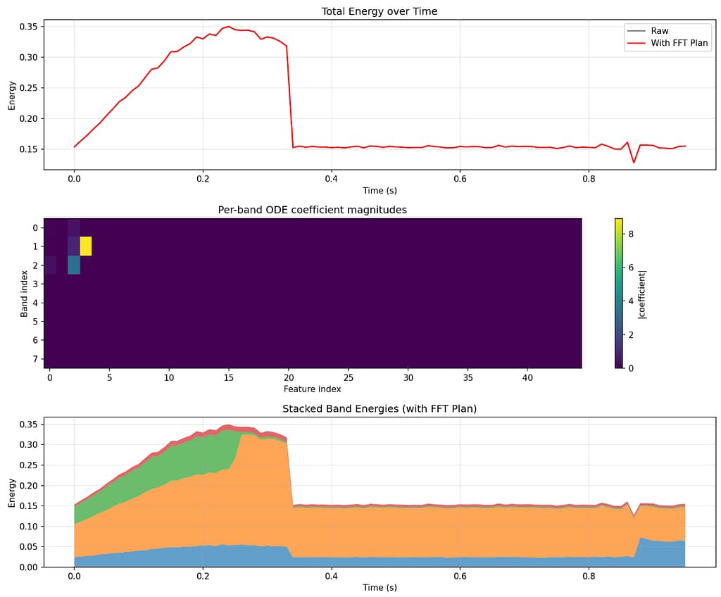
=== ODE Recovery Results ===
Mode: global

Band Influence Ranking:
Band (MHz)  Influence
   3.1-4.6  12.807979
   1.5-3.1   7.381399
   0.0-1.5   0.000000
   4.6-6.1   0.000000
   6.1-7.7   0.000000
   7.7-9.2   0.000000
  9.2-10.8   0.000000
 10.8-12.3   0.000000

Recovered ODE:
dY/dt = 0.721 + -7.381 E1 + 12.808 E2

Plot saved as 'fft_ode_band_mapping.png'

Done!

Global mode test complete.

Running in per-band mode...
RF Quantum SCYTHE Client FFT ODE Demo - 2025-09-02 16:55:57
API URL: http://localhost:8000
Per-band mode: True
Fetching FFT plan from http://localhost:8000/denoise/hints...
Warning: No FFT plan in response, using defaults

Generating synthetic RF data...
Generated 12288000 samples (1.0s at 12.288 MHz)

Computing band energies...
Computed 96 frames with 8 bands

Applying FFT plan...
Applied FFT plan with shift_bins=0

Recovering ODE from band energies...

=== Per-Band ODE Recovery Results ===
Mode: per_band
Recovered ODEs for 8 bands

Plot saved as 'fft_ode_band_mapping.png'

Done!

Per-band mode test complete../test_client_fft_ode_demo.sh
Starting API server in the background...
Server started with PID 565343
Server is ready
=== Testing RF Quantum SCYTHE Client FFT ODE Demo ===

Running in global mode (default)...
RF Quantum SCYTHE Client FFT ODE Demo - 2025-09-02 16:55:53
API URL: http://localhost:8000
Per-band mode: False
Fetching FFT plan from http://localhost:8000/denoise/hints...
Warning: No FFT plan in response, using defaults

Generating synthetic RF data...
Generated 12288000 samples (1.0s at 12.288 MHz)

Computing band energies...
Computed 96 frames with 8 bands

Applying FFT plan...
Applied FFT plan with shift_bins=0

Recovering ODE from band energies...

=== ODE Recovery Results ===
Mode: global

Band Influence Ranking:
Band (MHz)  Influence
   3.1-4.6  12.807979
   1.5-3.1   7.381399
   0.0-1.5   0.000000
   4.6-6.1   0.000000
   6.1-7.7   0.000000
   7.7-9.2   0.000000
  9.2-10.8   0.000000
 10.8-12.3   0.000000

Recovered ODE:
dY/dt = 0.721 + -7.381 E1 + 12.808 E2

Plot saved as 'fft_ode_band_mapping.png'

Done!

Global mode test complete.

Running in per-band mode...
RF Quantum SCYTHE Client FFT ODE Demo - 2025-09-02 16:55:57
API URL: http://localhost:8000
Per-band mode: True
Fetching FFT plan from http://localhost:8000/denoise/hints...
Warning: No FFT plan in response, using defaults

Generating synthetic RF data...
Generated 12288000 samples (1.0s at 12.288 MHz)

Computing band energies...
Computed 96 frames with 8 bands

Applying FFT plan...
Applied FFT plan with shift_bins=0

Recovering ODE from band energies...

=== Per-Band ODE Recovery Results ===
Mode: per_band
Recovered ODEs for 8 bands

Plot saved as 'fft_ode_band_mapping.png'

Done!

Per-band mode test complete.