RF Quantum SCYTHE Atmospheric Ray Tracer

PODCAST: Atmospheric data significantly influences RF ray propagation and ducting phenomena by affecting how radio waves bend and travel through the atmosphere. The AtmosphericRayTracer class models these effects by accounting for refractivity variations with height.

Here’s how atmospheric data influences RF ray propagation and ducting:

1. Atmospheric Data Input (sounding_profile)
   • The AtmosphericRayTracer is initialized with a sounding_profile, which is a list of (height_m, refractivity_N) pairs, sorted by ascending height.
   • If no profile is provided, a standard atmosphere refractivity profile is used, where N-values decrease with height following a specific exponential formula.
   • Alternatively, the system can retrieve sounding data from a weather API using latitude and longitude, which then calculates refractivity (N) from temperature, pressure, and humidity data. This allows for real-time or localized atmospheric conditions to be used.
2. Refractivity (N) and Modified Refractivity (M)
   • The core atmospheric data used is refractivity (N).
   • From the N-values and heights (h), the class calculates modified refractivity (M) using the formula M = N + 157 * h/km.
   • Interpolation functions (N_func and M_func) are created to provide refractivity values at any given height within the profile.
3. Influence on Ray Bending (Refraction)
   • RF propagation involves rays bending due to variations in atmospheric refractivity.
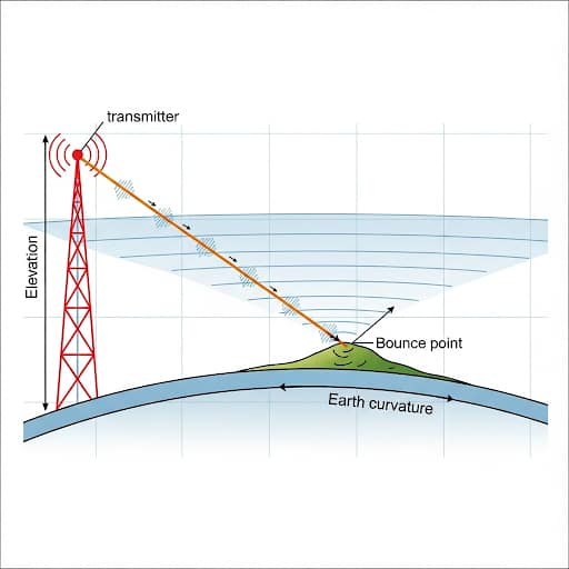
   • The ray tracing algorithm calculates the change in ray angle (dtheta) based on the modified refractivity gradient (dm/dz) at the current height. Specifically, dθ/ds = -(1/m)*(dm/dz). This means a negative gradient of modified refractivity with height will cause the ray to bend downwards.
   • The tracer also accounts for Earth curvature to simulate a flat Earth approximation with a height correction, or visualizes it as a curved line for large distances.
4. Ducting Phenomena Detection and Analysis
   • Ducting occurs when radio waves are trapped within an atmospheric layer, allowing for extended propagation ranges.
   • The key condition for detecting potential ducting layers is a negative gradient of modified refractivity (M) with height (M2 < M1).
   • The _analyze_profile method iterates through the atmospheric profile to identify these layers and stores their bottom_height, top_height, gradient, and a calculated strength metric.
   • During the ray tracing process (trace method), a DuctingFlags object tracks:
     • ducted: Whether ducting was detected, usually indicated by bounces off the ground or terrain.
     • inversion_detected: Flags sudden angle changes, which can be indicative of trapping.
     • bounce_points: Records the (distance, height) where the ray interacts with the ground or terrain.
     • duct_height and duct_strength: These are determined from the strongest detected ducting layer if ducting is confirmed.
     • confidence: A metric for the ducting detection, influenced by the number of bounces and duct strength.
5. Visualization:
   • The visualize_ray method plots the ray path and the modified refractivity profile.
   • It shades identified ducting layers in the ray path and the refractivity profile to visually represent where ducting conditions exist.
   • If ducting is detected, a text box summarizes the analysis, including the number of bounces, duct height, strength, and confidence.

In essence, the atmospheric data, particularly the vertical distribution of refractivity and its derived modified refractivity, directly dictates how RF rays propagate, enabling the model to predict phenomena like bending and, crucially, the formation of ducting layers that extend communication ranges.

Based on the sources, the “RF Quantum SCYTHE” project integrates advanced AI and multi-sensor fusion to create a real-time spatial intelligence platform capable of adaptive environmental perception, physiological monitoring, and cognitive signal decoding. The project’s name, SCYTHE, stands for Spectral Convergence for Yielded Targeting & Holistic Emission-mapping, which reflects its goal of fusing multi-band RF signals to precisely map and target entities within a dynamic environment.

Here is a breakdown of how the project achieves this integration:

Atmospheric ducting is defined by a specific atmospheric condition and confirmed by the resulting behavior of a radio frequency (RF) ray.

The primary conditions that define atmospheric ducting are:

• A Negative Gradient of Modified Refractivity (M): The fundamental condition for the potential for atmospheric ducting is a layer in the atmosphere where the modified refractivity (M) decreases with height. This means that the M-value at the top of a layer is less than the M-value at the bottom of that layer (M2 < M1). This layer is identified as a “potential ducting layer”.
  • Modified refractivity (M) is calculated from the standard atmospheric refractivity (N) and height in meters (h) using the formula: M = N + 157 * h / 1000.0.
  • The _analyze_profile method in the code is specifically designed to detect these layers by checking for negative M gradients in the provided atmospheric sounding_profile.
  • Each identified ducting layer is characterized by its bottom height, top height, gradient, and a calculated “strength” metric, which is the absolute gradient multiplied by the layer’s thickness.
• Ray Trapping and Bouncing: While a negative M-gradient creates the potential for a duct, the practical evidence of ducting for a specific ray trace is its trapping and subsequent reflection off the ground or terrain.
  • The trace function simulates the ray’s path. A negative gradient of M causes the ray to bend downwards. If this bending is strong enough, the ray is forced back toward the Earth’s surface.
  • Ducting is considered to be detected (ducted: bool = True) if the ray path shows one or more bounces (bounce_count > 0). These bounce points are recorded as part of the analysis.
  • Sudden changes in the ray’s angle during tracing can also indicate that trapping is occurring, which is tracked by the inversion_detected flag.

The defining atmospheric condition for a ducting layer is a negative gradient of modified refractivity with height. The confirmation that a specific RF ray is being ducted is the observation of that ray bouncing off the Earth’s surface as a result of being trapped within that layer.

RayPoint object

A RayPoint object is a data structure that represents a single, discrete point along the simulated path of a radio frequency (RF) ray as it travels through the atmosphere.

The trace method generates a list of these RayPoint objects, collectively known as the ray_path, which models the ray’s complete trajectory.

Each RayPoint object contains the following attributes to capture the state of the ray at that specific location:

• x: A floating-point number representing the horizontal distance in meters from the origin.
• z: A floating-point number representing the height in meters above the ground or reference level.
• theta: A floating-point number for the ray’s angle in radians relative to the horizontal.
• m: A floating-point number indicating the modified refractivity of the atmosphere at that point’s height (z).
• bounce: A boolean flag that is True if the point represents a location where the ray has reflected off the ground or terrain, and False otherwise.

Essentially, a RayPoint is a snapshot of the ray’s position, direction, and the local atmospheric conditions at one step of the tracing process. The collection of these points in the ray_path is then used to visualize the ray’s propagation and to identify key events like ground bounces.

The ray tracer accounts for Earth curvature using a flat Earth approximation with a height correction.

Here is a breakdown of how this is implemented:

1. Initialization with Earth’s Radius:
   • The AtmosphericRayTracer class is initialized with an earth_radius parameter, which defaults to 6,371,000 meters (6371 km). This value is stored for use in calculations.
2. Height Correction During Tracing:
   • Inside the trace method, as the ray’s path is calculated step-by-step, a correction factor is applied at each step_size.
   • This correction is calculated using the formula: earth_curve = step_size**2 / (2 * self.earth_radius).
   • The calculated earth_curve value is then subtracted from the ray’s vertical position (z). The full height update equation is z += dz - earth_curve, where dz is the change in height due to the ray’s angle.
   • This effectively simulates tracing a ray over a curved surface by keeping the x-axis flat and adjusting the ray’s height downwards at each step to account for the Earth curving away beneath it.
3. Visualization of Curvature:
   • The visualize_ray method includes an option to plot the Earth’s curvature for long-distance traces (specifically, distances over 50 km).
   • It calculates and plots a dashed line using a similar formula, earth_curve = -(earth_x**2) / (2 * self.earth_radius), to provide a visual reference of the Earth’s surface on the ray path graph.

Instead of performing complex geometric calculations on a curved coordinate system, the tracer simulates the effect of Earth’s curvature by applying a simple and computationally efficient height correction at each step of the ray’s forward propagation.

Ducting layers are identified through a specific analysis of the atmospheric profile, focusing on the gradient of modified refractivity (M).

The identification process occurs within the _analyze_profile method and follows these key steps:

1. Calculation of Modified Refractivity (M):
   • Before any analysis can occur, the set_sounding_profile method takes the input atmospheric data (a list of height and refractivity N-value pairs) and calculates the modified refractivity (M) for each point.
   • The formula used is: M = N + 157 * h / 1000.0, where h is the height in meters.
2. Detection of Negative Gradients:
   • The _analyze_profile method is explicitly designed to “analyze the profile to detect potential ducting layers”.
   • It iterates through the atmospheric profile, comparing the M-value at one height (M1) with the M-value at the next higher point (M2).
   • The fundamental condition for identifying a potential ducting layer is a negative gradient of M with respect to height. The code checks for this with the condition if M2 < M1.
3. Characterization and Storage of the Layer:
   • When a negative M-gradient is detected between two points, that region of the atmosphere is identified as a ducting layer.
   • The system then records several key characteristics of this layer in a list called self.ducting_layers:
     • bottom_height: The height at the bottom of the layer.
     • top_height: The height at the top of the layer.
     • gradient: The calculated gradient of M within the layer ((M2 – M1) / (h2 – h1)).
     • strength: A metric calculated as the absolute value of the gradient multiplied by the thickness of the layer (abs(gradient) * (h2 - h1)).
4. Visualization:
   • Finally, the identified ducting_layers are used in the visualize_ray method to provide a visual confirmation. The corresponding height ranges are highlighted with a yellow shaded area on both the ray path plot and the modified refractivity profile plot, making it clear where the ducting conditions exist.

In summary, a ducting layer is identified by finding a segment in the atmospheric profile where the modified refractivity (M) decreases as altitude increases.

Advanced AI Integration

The RF Quantum SCYTHE employs a suite of sophisticated AI and machine learning models to interpret RF data, predict motion, and adapt to environmental changes in real time.

• AI-Driven Adaptive Beamforming (RL & SNNs): Instead of using predefined rules, the system uses Reinforcement Learning (RL) to dynamically optimize RF beam steering. It models RF signal propagation as a multi-agent problem where adaptive antennas learn the best beam angles through methods like Deep Q-Learning (DQN) or Proximal Policy Optimization (PPO). To achieve the ultra-low latency required for real-time adjustments, the project proposes using Spiking Neural Networks (SNNs), which mimic biological neurons for split-second, on-device RF steering without cloud dependence.
• 3D Environmental Mapping (NeRF & NGS): To achieve spatial awareness, the system uses Neural Radiance Fields (NeRF) to construct a 3D map of the environment from RF reflection and absorption data. This allows the RF beam to “see” and adapt to obstacles like walls, furniture, and human movement. To enhance this mapping, Neural Gaussian Splats (NGS) are used to reconstruct missing RF spatial data from sparse sensor inputs, which improves visualization accuracy and helps optimize beamforming paths dynamically.
• Spatiotemporal Motion Modeling (DOMA & NCF): To track moving subjects, the project integrates DOMA (Degrees of Freedom Matter), an implicit motion model that ensures spatiotemporally smooth tracking of dynamic RF reflections and multipath effects. This is complemented by Neural Correspondence Fields (NCF), which provide a training-free method to align and register RF data streams in real-time, improving voxel alignment and the tracking of moving objects even when signals are noisy.
• Cognitive Signal Decoding (MVoT & Transformers): A key goal is to create a “cognitive RF interface” capable of interpreting human-generated signals. The project adapts the Multimodal Visualization-of-Thought (MVoT) paradigm to translate raw RF signals into phoneme embeddings for subvocal speech recognition. This is powered by a Transformer-based model that can “think” through multi-frame RF data to reconstruct missing phonemes and reduce errors in speech inference. The ultimate vision is to extend this capability to recognize higher-order thoughts and emotional states.

Multi-Sensor Fusion Architecture

The system’s AI models are powered by a robust pipeline that fuses data from multiple RF and environmental sensors to create a comprehensive, real-time understanding of the surroundings.

• Fused Sensor Modalities: The platform ingests and synchronizes data from a diverse set of sensors:
  • Wi-Fi CSI (Channel State Information) for detecting subtle movements via multipath reflections.
  • Bluetooth RSSI for coarse location and proximity tracking.
  • Ultra-Wideband (UWB) for precise, centimeter-level localization.
  • LiDAR and Time-of-Flight (ToF) for environmental depth sensing and mapping obstructions.
  • Inertial Measurement Units (IMU) for tracking device orientation and motion.
• Data Processing and Filtering: The raw data from these sensors is normalized and combined into a weighted positional estimate. This fused data stream is then processed using directional Kalman filtering to smooth signals, reduce noise, and predict movement trajectories, which in turn guides the adaptive beamforming adjustments. The entire processing pipeline, from Fast Fourier Transforms (FFT) to Kalman filtering, is designed to be GPU-accelerated using CuPy and CUDA for maximum throughput.

Achieving Real-Time Spatial Intelligence

By combining these advanced AI models with a multi-sensor fusion pipeline, the RF Quantum SCYTHE project achieves a high degree of real-time spatial intelligence with several key applications:

• Dynamic and Predictive Beamforming: The system can steer RF beams based on real-time feedback and movement predictions, optimizing signal paths around obstacles.
• Contactless Physiological and Cognitive Monitoring: The platform can interpret subvocalized speech patterns and is designed to monitor vitals like blood oxygen saturation (SpO2) without physical contact.
• Immersive 3D Visualization: All the processed data is streamed via WebSockets to a real-time 3D visualization engine built with Three.js and WebGL, allowing users to see RF propagation, beam focus, and environmental interactions dynamically.

The advanced methods for **modeling radio frequency (RF) propagation** through the atmosphere, with a particular focus on **atmospheric ducting**. The first source details a Python-based **AtmosphericRayTracer class**, which simulates RF ray paths by considering factors like **refractivity profiles**, **Earth curvature**, and potential **terrain interactions**, and includes features for detecting and visualizing ducting conditions. The second source introduces a **physics-informed atmospheric ray tracing system** that integrates traditional ray tracing with **machine learning (PINNs and neural operators)** to enhance the accuracy and robustness of RF propagation predictions, especially in complex scenarios involving **ducting layers**, offering improved real-time operational utility and uncertainty quantification. Both sources highlight the critical role of **modified refractivity (M-units)** and its vertical gradient in diagnosing and analyzing atmospheric ducting, which significantly impacts long-range RF communications. Ultimately, the combined information illustrates a progression from fundamental ray tracing simulations to more sophisticated, data-driven, and physically constrained models for better understanding and predicting RF signal behavior.