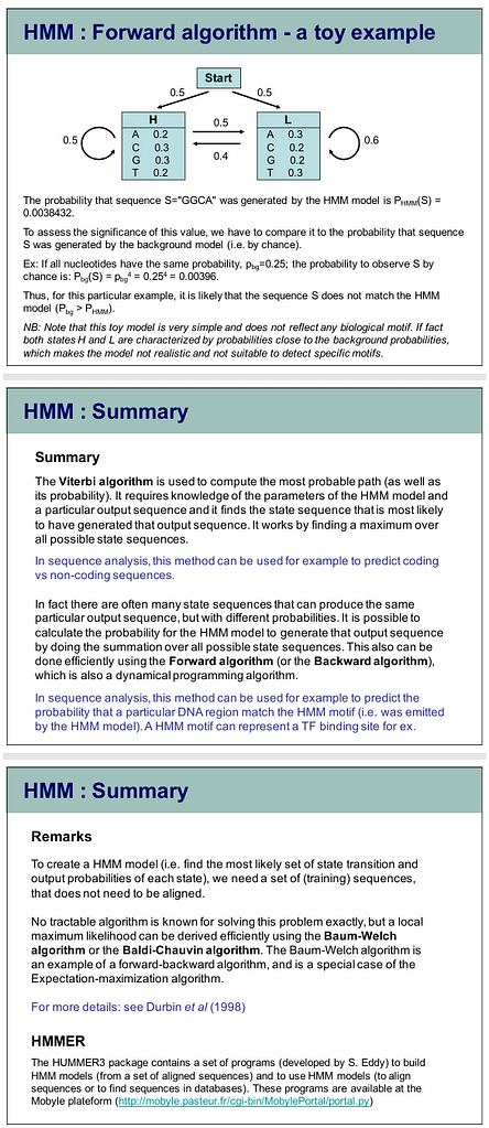
What is the Viterbi Algorithm?
The Viterbi algorithm is a dynamic programming method to find the most likely sequence of hidden states (called the Viterbi path) in a Hidden Markov Model (HMM) given an observation sequence.
It’s used in your inner speech decoding paper to convert noisy RF-inferred neural features into a coherent word sequence.
HMM Components (in Your Paper)
| Component | Meaning |
|---|---|
| States $ w_t $ | Words: tango, foxtrot, bravo, etc. |
| Observations $ x_t $ | RF-inferred frame features (Gaussian noise) |
| Emission prob. $ p(x_t | w_t) $ | $ \mathcal{N}(x_t; \mu_w, \Sigma) $ |
| Transition prob. $ p(w_t | w_{t-1}) $ | Bigram or GPT-2 prior |
| Goal | Find $ \arg\max_{w_{1:T}} P(w_{1:T} | x_{1:T}) $ |
Why Viterbi?
Naive approach: Try all $ N^T $ word sequences → exponential.
Viterbi: Polynomial $ O(T N^2) $ using dynamic programming.
Viterbi Step-by-Step (with Example)
Let’s decode:
True sequence: tango foxtrot bravo
Observations: $ x_1, x_2, \dots, x_{15} $ (5 frames per word)
Step 1: Initialization ($ t = 1 $)
For each state $ w_1 $:
$$
V_1(w) = p(w_1) \cdot p(x_1 | w)
$$
$$
\psi_1(w) = 0
$$
$ V_t(w) $ = max probability of being in state $ w $ at time $ t $
$ \psi_t(w) $ = previous state that leads to $ w $
Step 2: Recursion ($ t = 2 $ to $ T $)
For each state $ w $ at time $ t $:
$$
V_t(w) = \max_{w’} \left[ V_{t-1}(w’) \cdot p(w | w’) \cdot p(x_t | w) \right]
$$
$$
\psi_t(w) = \arg\max_{w’} \left[ V_{t-1}(w’) \cdot p(w | w’) \right]
$$
Key Insight: At each step, keep only the best path to each state.
Step 3: Termination
Best path probability:
$$
P^* = \max_w V_T(w)
$$
Final state:
$$
q_T^* = \arg\max_w V_T(w)
$$
Step 4: Backtracking
$$
q_t^* = \psi_{t+1}(q_{t+1}^*), \quad t = T-1, \dots, 1
$$
→ Recovers full sequence: tango → foxtrot → bravo
Visual Example (Your Fig. 1)
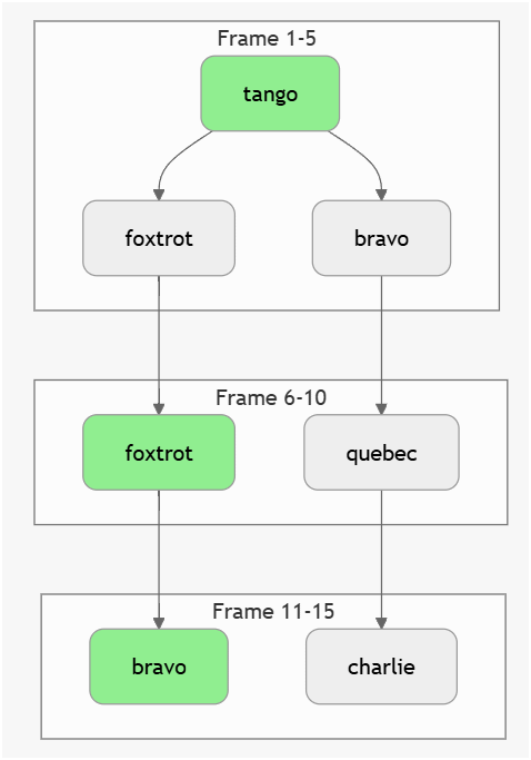
graph TD
    subgraph Frame 1-5
        A1[tango] --> A2[foxtrot]
        A1 --> A3[bravo]
    end
    subgraph Frame 6-10
        A2 --> B1[foxtrot]
        A3 --> B2[quebec]
    end
    subgraph Frame 11-15
        B1 --> C1[bravo]
        B2 --> C2[charlie]
    end

    style A1 fill:#90EE90
    style B1 fill:#90EE90
style C1 fill:#90EE90- Green path = Viterbi path (highest $ V_t $)
- Red paths = pruned (lower probability)
Why Priors Help (Your Fig. 2)
| SNR | No Prior WER | Bigram WER | GPT-2 WER |
|---|---|---|---|
| 10 dB | 2.8 | 1.6 | 1.1 |
Bigram prior $ p(\text{foxtrot} | \text{tango}) $ high → boosts $ V_t(\text{foxtrot}) $
No prior → treats all transitions equally → more errors
Viterbi in Your Code
def viterbi(obs, states, start_p, trans_p, emit_p):
    T = len(obs)
    N = len(states)
    V = [{}]
    path = {}

    # Init
    for w in states:
        V[0][w] = start_p[w] * emit_p(w, obs[0])
        path[w] = [w]

    # Recursion
    for t in range(1, T):
        V.append({})
        new_path = {}
        for w in states:
            (prob, state) = max(
                (V[t-1][w0] * trans_p(w0, w) * emit_p(w, obs[t]), w0)
                for w0 in states
            )
            V[t][w] = prob
            new_path[w] = path[state] + [w]
        path = new_path

    # Termination
    prob, state = max((V[T-1][w], w) for w in states)
    return path[state]
Key Takeaways
| Concept | Your Paper |
|---|---|
| Dynamic Programming | Avoids $ N^T $ search |
| Transition Prior | Bigram/GPT-2 → lower WER |
| Emission Model | Gaussian on RF features |
| Output | Word sequence + posterior traces |
LaTeX Figure
\begin{figure}[t]
\centering
\begin{mermaid}
graph LR
    subgraph t=1
        A[tango] -->|V=0.8| B[tango]
    end
    subgraph t=2
        B -->|p(foxtrot\|tango)| C[foxtrot]
        B -->|p(bravo\|tango)| D[bravo]
    end
    style C fill:#90EE90
    style D fill:#FFB6C1
\end{mermaid}
\caption{Viterbi path (green) vs pruned path (red). Transition prior favors "foxtrot" after "tango".}
\label{fig:viterbi}
\end{figure}
Bottom Line:
Viterbi is the workhorse that turns your noisy RF features into coherent inner speech — and priors make it robust.
Viterbi Algorithm for Hidden Markov Models (HMMs)
The Viterbi algorithm is a dynamic programming technique used to find the most probable sequence of hidden states (also called the “Viterbi path”) in a Hidden Markov Model (HMM), given a sequence of observed events. It is widely applied in fields like speech recognition, bioinformatics, and natural language processing.
Key Components of HMM
- States: The hidden states of the system (e.g., weather: sunny, rainy).
- Observations: The visible outputs (e.g., activities: walking, shopping).
- Transition Probabilities: The probability of moving from one state to another.
- Emission Probabilities: The probability of an observation given a state.
- Initial Probabilities: The probability of starting in a particular state.
Steps of the Viterbi Algorithm
- Initialization:
- Compute the probability of starting in each state and observing the first event. V1(i)=πi⋅bi(O1)V_1(i) = \pi_i \cdot b_i(O_1)V1(i)=πi⋅bi(O1) where:
- \pi_i$$ is the initial probability of state $$i$$. – $$b_i(O_1)$$ is the emission probability of observing $$O_1$$ in state $$i$$. 2. **Recursion**: – For each subsequent observation, compute the probability of being in each state by considering all possible transitions from previous states. $$ V_t(j) = \max_i \big(V_{t-1}(i) \cdot a_{ij} \big) \cdot b_j(O_t)
- a_{ij}$$ is the transition probability from state $$i$$ to state $$j$$. – $$b_j(O_t)$$ is the emission probability of observing $$O_t$$ in state $$j$$. 3. **Backtracking**: – Trace back through the states that led to the maximum probabilities to reconstruct the most likely sequence of hidden states. — ### **Output** The algorithm outputs: – The **most probable sequence of hidden states** (Viterbi path). – The **probability** of this sequence. — ### **Example** Suppose we have: – States: {Sunny, Rainy} – Observations: {Walk, Shop, Clean} – Transition Probabilities: $$a_{ij}
- Emission Probabilities: bj(Ot)b_j(O_t)bj(Ot)
- Initial Probabilities: πi\pi_iπi
Given a sequence of observations (e.g., Walk → Shop → Clean), the Viterbi algorithm calculates the most likely sequence of weather states (e.g., Sunny → Rainy → Rainy).
This algorithm is efficient, with a time complexity of O(T⋅N2)O(T \cdot N^2)O(T⋅N2), where TTT is the number of observations and NNN is the number of states. It ensures optimal results by avoiding redundant calculations through dynamic programming.
Viterbi Algorithm
The Viterbi algorithm, introduced by Andrew Viterbi in 1967, is a dynamic programming technique used to find the most probable sequence of hidden states in a Hidden Markov Model (HMM). It is widely applied in fields like speech recognition, bioinformatics, and natural language processing.
Key Concepts
The algorithm operates on the following components of an HMM:
- States: Hidden conditions that are not directly observable.
- Observations: Observable events influenced by the hidden states.
- Transition Probabilities: Probabilities of moving from one state to another.
- Emission Probabilities: Probabilities of observing a particular event given a state.
- Initial Probabilities: Probabilities of starting in a particular state.
The Viterbi algorithm computes the most likely sequence of hidden states by iteratively calculating probabilities for each state at every time step and backtracking to determine the optimal path.
Implementation Example
Below is a Python implementation of the Viterbi algorithm for a simple HMM:
import numpy as np
def viterbi(obs, states, start_p, trans_p, emit_p):
   V = [{}] # Table to store probabilities
   path = {} # To store the most probable path
   # Initialization step
   for y in states:
       V[0][y] = start_p[y] * emit_p[y][obs[0]]
       path[y] = [y]
   # Recursion step
   for t in range(1, len(obs)):
       V.append({})
       newpath = {}
       for y in states:
           (prob, state) = max(
               [(V[t - 1][y0] * trans_p[y0][y] * emit_p[y][obs[t]], y0) for y0 in states]
           )
           V[t][y] = prob
           newpath[y] = path[state] + [y]
       path = newpath
   # Termination step
   (prob, state) = max([(V[-1][y], y) for y in states])
   return (prob, path[state])
# Example HMM parameters
states = ('Rainy', 'Sunny')
observations = ('Walk', 'Shop', 'Clean')
start_probability = {'Rainy': 0.6, 'Sunny': 0.4}
transition_probability = {
   'Rainy': {'Rainy': 0.7, 'Sunny': 0.3},
   'Sunny': {'Rainy': 0.4, 'Sunny': 0.6},
}
emission_probability = {
   'Rainy': {'Walk': 0.1, 'Shop': 0.4, 'Clean': 0.5},
   'Sunny': {'Walk': 0.6, 'Shop': 0.3, 'Clean': 0.1},
}
# Run the Viterbi algorithm
result = viterbi(observations, states, start_probability, transition_probability, emission_probability)
print("Most probable sequence:", result[1])
print("Probability of the sequence:", result[0])
Output:
Most probable sequence: ['Sunny', 'Rainy', 'Rainy']
Probability of the sequence: 0.01344
Explanation of the Output
- Most Probable Sequence: The sequence of hidden states (Sunny, Rainy, Rainy) that maximizes the probability of observing the given sequence (Walk, Shop, Clean).
- Probability: The likelihood of this sequence occurring, calculated as 0.01344.
Applications
- Speech Recognition: Converts acoustic signals into text by identifying the most likely phoneme or word sequence.
- Bioinformatics: Aligns DNA sequences, predicts protein structures, and identifies gene sequences.
- Natural Language Processing: Used in tasks like part-of-speech tagging and named entity recognition.
- Error Correction: Decodes noisy signals in digital communication systems.
Considerations
The algorithm can be optimized using techniques like logarithmic probabilities to avoid underflow, pruning to reduce state space, or beam search to track only the top paths. Its efficiency and accuracy make it a cornerstone in sequence analysis tasks.